library_size

Functions to estimate the total library size (number of unique genotypes) from sampling data. Fits a hybrid power-law distribution model to genotype frequency data and extrapolates to estimate unobserved genotypes.

---

source

estimate_library_size

def estimate_library_size(
    observed_counts:list, G:int, # total number of possible unique genotypes
    N:int, # number of cells
    verbose:bool=False
)->dict:

Estimates the expected number of unique genotypes sampled (K_N).

This function uses a hybrid model: 1. The “head” (high-frequency genotypes) uses empirical probabilities. 2. The “tail” (low-frequency and unobserved genotypes) is modeled with a power-law (Zipf) distribution.

Args: observed_counts (list[int]): A list of UMI counts for each observed unique genotype. G (int): The total number of possible unique genotypes. N (int): The number of cells in the culture to sample from.

Returns: dict: A dictionary containing the results: ‘E_KN’ (float): The final estimated E[K_N]. ‘B’ (int): The estimated breakpoint. ‘alpha’ (float): The estimated power-law exponent. ‘E_head’ (float): The contribution to E[K_N] from the head. ‘E_tail’ (float): The contribution to E[K_N] from the tail.

---

source

find_best_breakpoint

def find_best_breakpoint(
    counts:ndarray
)->tuple:

Finds the optimal breakpoint B for a hybrid power-law distribution.

This function iterates through possible breakpoints and performs a linear regression on the log-log plot of the tail of the distribution (rank vs. probability). The optimal breakpoint is chosen as the one that maximizes the R-squared value of the linear fit, indicating the point where the power-law behavior is most pronounced.

Args: counts (np.ndarray): An array of UMI counts for each observed genotype, sorted in descending order.

Returns: tuple[int, float, float]: A tuple containing: - best_b (int): The estimated optimal breakpoint B. - best_alpha (float): The estimated power-law exponent alpha for the tail. - best_intercept (float): The intercept from the log-log linear regression.

from dgrec.example_data import get_example_data_dir

data_path=get_example_data_dir()
gen_list=parse_genotypes(os.path.join(data_path,"sacB_genotypes.csv"))

read_ref_file="sacB_ref.fasta"
ref=next(SeqIO.parse(os.path.join(data_path,read_ref_file),"fasta"))
ref_seq=str(ref.seq)

#showing a few example lines
for g,n in gen_list[1:200:20]:
    print(n,"\t",g)

279      A91G
28   A68C
15   A72G,A79T,A91T
10   A61G,A72G
6    A61G,A68G
6    A68G,A76G,A91G
5    A61T,A79G
4    A86T
4    A72G,A76G,A86G,A91T
3    A61T,A76G,A91G

# Demo: find_best_breakpoint
counts_demo = np.sort(np.array([c for g,c in gen_list], dtype=np.float64))[::-1]
counts_demo = np.trim_zeros(counts_demo)
B, alpha, intercept = find_best_breakpoint(counts_demo)
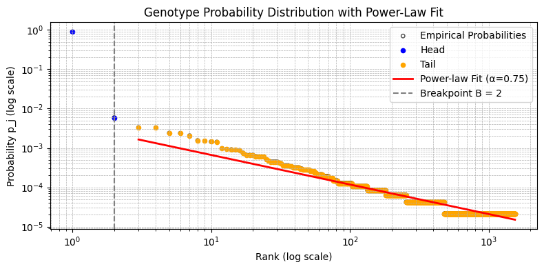
print(f"Breakpoint B={B}, alpha={alpha:.4f}, intercept={intercept:.4f}")

Breakpoint B=2, alpha=0.7513, intercept=-5.5858

counts = [c for g,c in gen_list]
results = estimate_library_size(counts, G=4**20, N=10**9)
results

{'library_size': 89740015,
 'B': 2,
 'alpha': 0.7512643654095239,
 'C': 2.3011837490037884e-05,
 'intercept': -5.585815841202696,
 'E_head': 2.0,
 'E_tail': 89740013.23215128}

---

source

plot_distribution

def plot_distribution(
    counts:ndarray, results:dict
):

Plots the probability distribution on a log-log scale.

Args: counts (np.ndarray): Sorted array of observed genotype counts. results (dict): The dictionary returned by estimate_expected_genotypes.

plot_distribution(counts, results)

Displaying plot...